Affinity segmentation
This is the term that I think best describes encoding an image segmentation it its most general, information-dense form: an affinity graph. To explain what this is, we will first consider two cells in contact.
The hierarchy of segmentation encoding
Show code cell source
  1# Load image and masks
  2import string
  3import matplotlib as mpl
  4import matplotlib.pyplot as plt
  5mpl.rcParams['figure.dpi'] = 600
  6# mpl.rcParams['facecolor'] = [0]*4
  7
  8plt.rc('figure', facecolor=[0]*4)
  9
 10plt.style.use('dark_background')
 11mpl.use('Agg')
 12
 13%matplotlib inline
 14
 15from pathlib import Path
 16import os
 17from cellpose_omni import io, plot
 18import fastremap
 19
 20import omnipose
 21omnidir = Path(omnipose.__file__).parent.parent.parent
 22basedir = os.path.join(omnidir,'docs','_static')
 23# name = 'ecoli_phase'
 24name = 'ecoli'
 25ext = '.tif'
 26image = io.imread(os.path.join(basedir,name+ext))
 27masks = io.imread(os.path.join(basedir,name+'_labels'+ext))
 28slc = omnipose.measure.crop_bbox(masks>0,pad=0)[0]
 29masks = fastremap.renumber(masks[slc])[0]
 30image = image[slc]
 31
 32# Plot a few things
 33
 34import matplotlib.pyplot as plt
 35from omnipose.plot import apply_ncolor, plot_edges, imshow
 36from omnipose import utils
 37import numpy as np
 38# import matplotlib_inline
 39# matplotlib_inline.backend_inline.set_matplotlib_formats('svg')
 40
 41from mpl_toolkits.axes_grid1.inset_locator import zoomed_inset_axes
 42from mpl_toolkits.axes_grid1.inset_locator import inset_axes
 43from mpl_toolkits.axes_grid1.inset_locator import mark_inset
 44from matplotlib.patches import Patch
 45
 46
 47
 48images = [image, masks>0, apply_ncolor(masks), masks>0]
 49labels = ['Image\n(phase contrast)', 'Semantic\nsegmentation',
 50          'Instance\nsegmentation', 'Affinity\nsegmentation']
 51
 52# Set up the figure and subplots
 53N = len(images)
 54
 55f = 1
 56Y,X = masks.shape[-2:]
 57M = 1
 58
 59h,w = masks.shape[-2:]
 60
 61sf = w
 62p = 0.0035*w # needs to be defined as fraction of width for aspect ratio to work?
 63h /= sf
 64w /= sf
 65
 66# Calculate positions of subplots
 67left = np.array([i*(w+p) for i in range(N)])*1.
 68bottom = np.array([0]*N)*1.
 69width = np.array([w]*N)*1.
 70height = np.array([h]*N)*1.
 71
 72max_w = left[-1]+width[-1]
 73max_h = bottom[-1]+height[-1]
 74
 75sw = max_w
 76sh = max_h
 77
 78sf = max(sw,sh)
 79left /= sw
 80bottom /= sh
 81width /= sw
 82height /= sh
 83
 84# Create figure
 85s = 6
 86fig = plt.figure(figsize=(s,s*sh/sw), frameon=False, dpi=300)
 87# fig.patch.set_facecolor([0]*4)
 88
 89# Add subplots
 90axes = []
 91for i in range(N):
 92    ax = fig.add_axes([left[i], bottom[i], width[i], height[i]])
 93    axes.append(ax)
 94
 95# Iterate over each subplot and set the image, label, and formatting
 96c =  [0.5]*3
 97fontsize = 11
 98
 99# bounds = [40,20,10,10]
100bounds = [11,22,8,8]
101h,w = masks.shape[-2:]
102extent = np.array([0,w,0,h])#-0.5
103
104
105sy,sx,wy,wx = bounds
106zoomslc = tuple([slice(sy,sy+wy),slice(sx,sx+wx)])
107
108
109cmap='inferno'
110
111zoom = 3
112# zoom, f = 5, 0.75
113color = [.75]*3
114edgecol = [1/3]*3
115edgecol = [.75]*3+[.5]
116axcol = [0.5]*3
117# edgecol = [.5,.75,0]+[2/3]
118
119lw= .2
120labelpad = 3
121fontsize2 = 8
122
123do_labels = 0
124
125for i, ax in enumerate(axes):
126
127    # inset axes
128    axins = zoomed_inset_axes(ax, zoom, loc='lower left',
129                              bbox_to_anchor=(-wx/w,-2*wy/h),
130                              # bbox_to_anchor=(-wx/w*zoom/2,-zoom*wy/h),
131                              # bbox_to_anchor=(-f*zoom*wy/h,-f*wx/w*zoom),
132
133
134                              bbox_transform=ax.transAxes)
135
136    if i==N-1:
137        # ax.invert_yaxis()
138
139        dim = masks.ndim
140        shape = masks.shape
141        steps, inds, idx, fact, sign = utils.kernel_setup(dim)
142        coords = np.nonzero(masks)
143        affinity_graph = omnipose.core.masks_to_affinity(masks, coords, steps,
144                                                         inds, idx, fact, sign, dim)
145        neighbors = utils.get_neighbors(coords,steps,dim,shape)
146        summed_affinity, affinity_cmap = plot_edges(shape,affinity_graph,neighbors,coords,
147                                                    figsize=1,fig=fig,ax=ax,extent=extent,
148                                                    edgecol=edgecol,cmap=cmap,linewidth=lw
149                                                   )
150
151
152        axins.invert_yaxis()
153        ax.invert_yaxis()
154
155        summed_affinity, affinity_cmap = plot_edges(shape,affinity_graph,neighbors,coords,
156                                            figsize=1,fig=fig,ax=axins,
157                                            extent=extent,
158                                            edgecol=edgecol,linewidth=lw*zoom,cmap=cmap,
159                                                    bounds=bounds
160                                           )
161
162        axins.set_xlim(zoomslc[1].start, zoomslc[1].stop)
163        axins.set_ylim(h-zoomslc[0].start, h-zoomslc[0].stop)
164
165
166        loc1,loc2 = 4,2
167        patch, pp1, pp2 = mark_inset(ax, axins, loc1=loc1, loc2=loc2, fc="none", ec=color+[1],zorder=2)
168        pp1.loc1 = 4
169        pp1.loc2 = 1
170        pp2.loc1 = 2
171        pp2.loc2 = 3
172
173
174        N = affinity_cmap.N
175        colors = affinity_cmap.colors
176
177        cax = inset_axes(ax, width="50%", height="100%", loc='lower right',
178                 bbox_to_anchor=(-.05, -0.7, 1, 1), bbox_transform=ax.transAxes,
179                 borderpad=0)
180
181        # Display the color swatches as an image
182        n = np.arange(3,9)
183        Nc = len(n)
184        cax.imshow(affinity_cmap(n.reshape(1,Nc)))#,vmin=n[0]-1,vmax=n[-1]+1)
185
186        # Set the y ticks and tick labels
187        cax.set_xticks(np.arange(Nc))
188        nums = [str(i) for i in n]
189        cax.set_xticklabels(nums,c=c,fontsize=fontsize2)
190        cax.tick_params(axis='both', which='both', length=0, pad=labelpad)
191        cax.set_yticks([])
192
193        wa = .07
194        ha = .05
195        cax.set_aspect(ha/wa)
196        cax.set_title('Connections',c=c,fontsize=fontsize2,pad=labelpad)
197        for spine in cax.spines.values():
198            spine.set_color(None)
199    else:
200
201        ax.imshow(images[i],cmap='gray',extent=extent)
202        # axins.imshow(images[i][zoomslc],extent=extent,origin='upper')
203        axins.imshow(images[i],extent=extent,cmap='gray')
204        # axins.imshow(images[i])#,extent=extent)
205
206        if i>0:
207            imp = masks[::-1][zoomslc]
208            if i==1:
209                imp = imp>0
210            for (j,k),label in np.ndenumerate(imp):
211                axins.text(k+sx+0.5, j+sy+0.45, int(label), ha='center', va='center', color=[(label==0)*0.5]*3,fontsize=4)
212
213
214        axins.set_xlim(zoomslc[1].start, zoomslc[1].stop)
215        axins.set_ylim(zoomslc[0].start, zoomslc[0].stop)
216
217        mark_inset(ax, axins, loc1=2, loc2=4, fc="none", ec=color+[1],zorder=2)
218
219
220    if do_labels:
221        ax.set_title(labels[i],c=c,fontsize=fontsize,fontweight="bold",pad=5)
222    else:
223        ax.annotate(string.ascii_lowercase[i], xy=(-0.1, 1), xycoords='axes fraction',
224        xytext=(0, 0), textcoords='offset points', va='top', c=axcol,
225        fontsize=fontsize)
226
227    ax.axis('off')
228    axins.set_xticks([])
229    axins.set_yticks([])
230    axins.set_facecolor([0]*4)
231
232    for spine in axins.spines.values():
233        spine.set_color(color)
234
235
236# plt.subplots_adjust(wspace=0.15)
237fig.patch.set_facecolor([0]*4)
238
239# Display the plot
240plt.show()
2025-06-27 15:54:59,673 [INFO] omnipose/gpu.py <module>....() line 12 On ARM, OMP_NUM_THREADS set to CPU core count = 1, PARLAY_NUM_THREADS set to 1.
masks (61, 56) uint8

Semantic segmentation sorts pixels into semantic classes. This is often just two classes, or binary classification: foreground and background. In this case, foreground is cell and background is media. As you can see, semantic segmentation does not discern between adjacent instances of foreground objects. We store a semantic segmentation as a binary image file with the same dimensions as the image itself, with foreground pixels labeled True (1) and background False (0).
Instance segmentation assigns a unique integer to the pixels each instance of an object - in this case, each cell. This is also conveniently stored as an image file, typically uint8 (unsigned 8-bit integer) for up to \(2^{8}-1=255\) labels or uint16 (unsigned 16-bit integer) for up to \(2^{16}-1=65535\) labels. Signed and/or unsigned 32- or 64-bit formats may also be used, but your OS may not be able to preview these files in its native file manager.
Note
Some instance labels use -1 as an "ignore" label. This can be in conflict with several tasks from indexing to label formatting, which assume unsigned integers, so care must be taken when working with signed formats (int) versus unsigned (uint).
Bad labels I: Semantic islands to instance labels
Semantic segmentation can be converted into instance segmentation, and this forms the basis of many instance segmentation pipelines. The general steps are:
Pre-process image: traditional filtering/blurring/feature extraction or DNN transformation
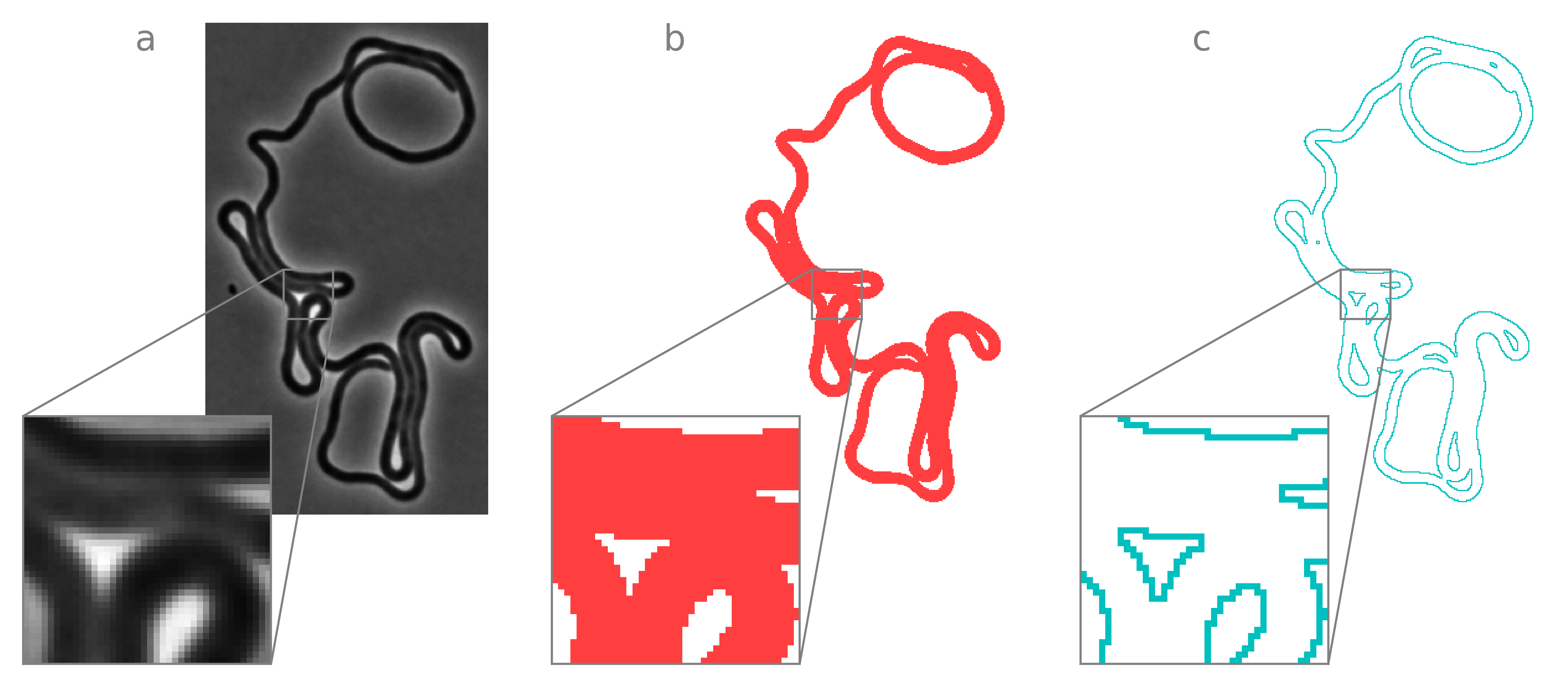
Threshold processed image: adaptive techniques are usually used on the pre-processed image to ensure that the majority of objects pixels are identified despite variations within an image and among images in a dataset. Importantly, object boundaries must not be identified as foreground. This allows each object to be associated with a unique island of foreground pixels.
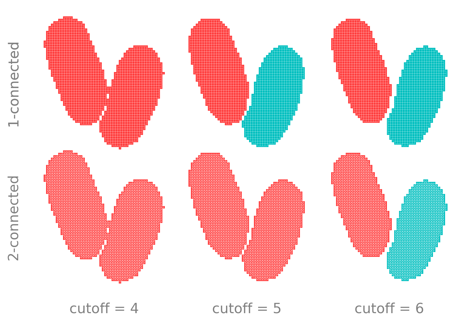
These unique blobs are identified using connected components labeling. This is the process of building an affinity graph, where pixels are nodes and edges are formed between any adjacent foreground pixels. Adjacency can be defined most narrowly by sharing edges (1-connected in Python, 4-connected in MATLAB) or more broadly by sharing either edges or vertices (2-connected in Python, 8-connected in MATLAB). The graph is then traversed to find all connected components of the graph.
These points are illustrated below. By simulating the amount of foreground pixels detected by filtering+thresholding, we see that is is impossible to distinguish between the two cells until much of the boundary is lost, particularly when using 2-connectivity.
Show code cell source
  1import skimage.measure
  2
  3connectivity = [1,2]
  4cutoffs = [4,5,6]
  5row_labels = ['{}-connected'.format(i) for i in connectivity]
  6col_labels = ['cutoff = {}'.format(i) for i in cutoffs]
  7# Define the grid dimensions
  8num_rows = len(row_labels)
  9num_cols = len(col_labels)
 10
 11# Create the grid of subplots
 12
 13# f = .75
 14# dpi = mpl.rcParams['figure.dpi']
 15# Y,X = masks.shape[-2:]
 16# szX = max(X//dpi,2)*f
 17# szY = max(Y//dpi,2)*f
 18# fig, axes = plt.subplots(num_rows, num_cols,figsize=(szX*num_cols,szY*num_rows))
 19
 20
 21
 22
 23h,w = masks.shape[-2:]
 24
 25sf = w
 26p = 0.05
 27h /= sf
 28w /= sf
 29
 30# Calculate positions of subplots
 31N = num_cols
 32M = num_rows
 33left = np.array([5*p+i*(w+p) for i in range(N)]*M).flatten().astype(float)
 34# bottom = np.array([1.5*p]*N + [h+p]*N).flatten().astype(float)
 35bottom = np.array([h+p]*N+[3*p]*N).flatten().astype(float)
 36width = np.array([[w]*N]*M).flatten().astype(float)
 37height = np.array([[h]*N]*M).flatten().astype(float)
 38
 39max_w = left[-1]+width[-1]
 40max_h = bottom[-1]+height[-1]
 41
 42sw = max_w
 43sh = max_h
 44
 45sf = max(sw,sh)
 46left /= sw
 47bottom /= sh
 48width /= sw
 49height /= sh
 50
 51# Create figure
 52s = 5
 53fig = plt.figure(figsize=(s,s*sh/sw), frameon=False, dpi=300,facecolor=[0]*4)
 54# fig.patch.set_facecolor([0]*4)
 55
 56# Add subplots
 57axes = []
 58for i in range(N*M):
 59    ax = fig.add_axes([left[i], bottom[i], width[i], height[i]])
 60    ax.set_facecolor([0]*4)
 61
 62    axes.append(ax)
 63
 64
 65fig.patch.set_facecolor([0]*4)
 66color = [0.5]*3
 67# for row,conn in enumerate(connectivity):
 68#     for col,cutoff in enumerate(cutoffs):
 69
 70for i,ax in enumerate(axes):
 71    row,col= np.unravel_index(i,(M,N))
 72
 73    cutoff = cutoffs[col]
 74    conn = connectivity[row]
 75
 76
 77    bin0 = summed_affinity>cutoff
 78    msk0 = skimage.measure.label(bin0,connectivity=conn)
 79    pic = apply_ncolor(msk0)
 80
 81
 82    dim = masks.ndim
 83    shape = masks.shape
 84    steps, inds, idx, fact, sign = utils.kernel_setup(dim)
 85    coords = np.nonzero(msk0)
 86    affinity_graph = omnipose.core.masks_to_affinity(msk0, coords, steps,
 87                                                     inds, idx, fact, sign, dim)
 88    neighbors = utils.get_neighbors(coords,steps,dim,shape)
 89
 90    #choose to plot cardinal connections only
 91    step_inds = None if conn==2 else inds[1]
 92
 93    # index = np.ravel_multi_index([[row],[col]],(N,M))
 94    # ax = axes[row*col]
 95    ax.axis('off')
 96
 97    # ax.text(0,0,i)
 98
 99    plot_edges(shape,affinity_graph,neighbors,coords,figsize=1,extent=extent,
100               fig=fig,ax=ax,step_inds=step_inds,pic=pic,origin='lower',edgecol=[1,1,1,0.5])
101
102    ax.invert_yaxis()
103
104    if i<N:
105        ax.annotate(col_labels[i], xy=(0.5, 1), xytext=(0, ax.xaxis.labelpad),
106                xycoords=ax.xaxis.label, textcoords='offset points',
107                ha='center', va='baseline',color=color,fontsize=fontsize)
108
109    if i%M==0:
110        ax.annotate(row_labels[row], xy=(0, 0), xytext=(-ax.yaxis.labelpad + 20, 0),
111                    xycoords=ax.yaxis.label, textcoords='offset points',
112                    ha='right', va='center', rotation=90,color=color,fontsize=fontsize)
113
114plt.show()
masks (61, 56) int32
masks (61, 56) int32
masks (61, 56) int32
masks (61, 56) int32
masks (61, 56) int32
masks (61, 56) int32
Although such sloppy segmentation is good enough for some tasks, we have a better tools now. So in general, do not use image thresholding for segmentation.
Bad labels II: Watershed lines
While we are on the topic, missing boundary pixels also frequently arise when applying the watershed transform. As usually implemented, this ubiquitous operation returns a semantic classification of an image into watershed lines and catchment basins. As you can tell by the above example, this means that distinct basins must be separated by a 1- or 2-connected watershed line, and therefore boundary pixels are always left unclassified.
There are implementations that allow users to return instance labels without the gaps let by watershed lines (e.g., skimage.segmentation.watershed), but I have yet to see a paper published using this method. Despite this fix, watershed also tends to over-segment images (even when transformed by traditional filters or DNNs). So in general, do not use watershed for instance segmentation.
Bad labels III: Self-contact boundaries
Instance labels are good enough to fully describe a lot of objects. More precisely, there is a bijective map between the affinity graph and the instance label matrix whenever all edge pixels are in contact with a non-self pixel. This assumption fails in many interesting (and biologically relevant) scenarios, including bacterial microscopy. Consider the following image containing one extremely filamentous cell and corresponding cell mask:
Show code cell source
  1# read in files; this is an entire movie, but we will just be looking at the last frame
  2import tifffile
  3
  4nm = 'long_10_2'
  5masks = tifffile.imread(os.path.join(basedir,nm+'_op_masks.tif'))
  6phase = tifffile.imread(os.path.join(basedir,nm+'_phase.tif'))
  7fluor = tifffile.imread(os.path.join(basedir,nm+'_fluor.tif'))
  8afnty = utils.load_nested_list(os.path.join(basedir,nm+'_affinity.npz'))
  9
 10# make figure
 11import omnipose, cellpose_omni
 12im = phase[-1]
 13msk = masks[-1]
 14
 15f = 1
 16c = [0.5]*3
 17fontsize=11
 18
 19titles = [r'$\bf{image}$'+'\n(phase contrast)', r'$\bf{label}$'+'\n(single cell mask)', r'$\bf{boundary}$'+'\n(from cell mask)']
 20ol = cellpose_omni.utils.masks_to_outlines(msk,omni=True)
 21# outlines = np.stack([ol]*4,axis=-1)*0.5
 22images = [im,
 23          omnipose.plot.apply_ncolor(msk),
 24          omnipose.plot.apply_ncolor(ol,offset=.5)]
 25
 26
 27
 28# Set up the figure and subplots
 29N = len(images)
 30h,w = im.shape
 31
 32sf = h
 33p = 0.5 # needs to be defined as fraction of width for aspect ratio to work?
 34
 35
 36h,w = im.shape
 37extent = np.array([0,w,0,h])#-0.5
 38sy,sx,wy,wx = [h//2.5,w//3.6,40,40]
 39zoomslc = tuple([slice(sy,sy+wy),slice(sx,sx+wx)])
 40zoom = 5
 41bbox_to_anchor = (-(wx/w)*zoom/(1.25),-zoom/1.5*wy/h) # inset axis
 42
 43
 44asp = h/w
 45
 46h /= sf
 47w /= sf
 48
 49oy,ox = np.abs(bbox_to_anchor)/2
 50# oy,ox = 0.,0.
 51# Calculate positions of subplots
 52left = np.array([ox+i*(w+p) for i in range(N)])*1.
 53bottom = np.array([oy]*N)*1.
 54width = np.array([w]*N)*1.
 55height = np.array([h]*N)*1.
 56
 57max_w = left[-1]+width[-1]+ox
 58max_h = bottom[-1]+height[-1]+oy
 59
 60sw = max_w
 61sh = max_h
 62
 63sf = max(sw,sh)
 64left /= sw
 65bottom /= sh
 66width /= sw
 67height /= sh
 68
 69# Create figure
 70s = 6.5
 71fig = plt.figure(figsize=(s,s*sh/sw), frameon=False, dpi=600)
 72# fig.patch.set_facecolor([0]*4)
 73
 74# Add subplots
 75axes = []
 76for i in range(N):
 77    ax = fig.add_axes([left[i], bottom[i], width[i], height[i]])
 78    axes.append(ax)
 79
 80
 81
 82lwa = 2/N # linewidth for axes
 83lw = lwa/20 # linewidth for affinity graph
 84labelpad = 2
 85
 86for i, ax in enumerate(axes):
 87
 88    ax.imshow(images[i],cmap='gray',extent=extent)
 89    ax.axis('off')
 90
 91
 92
 93    # inset axes....
 94    # axins = ax.inset_axes([0.5, 0.5, 0.47, 0.47])
 95    # axins = inset_axes(ax, 1,1 , loc=2, bbox_to_anchor=(.08, 0.35))
 96    axins = zoomed_inset_axes(ax, zoom, loc='lower left',
 97                              # bbox_to_anchor=(1.1, 1.1),
 98                              # bbox_to_anchor=(-.15,-.15),
 99                              bbox_to_anchor=bbox_to_anchor,
100                              bbox_transform=ax.transAxes)
101
102
103
104    # axins.imshow(images[i][zoomslc],extent=extent,origin='upper')
105    axins.imshow(images[i],extent=extent,cmap='gray')
106    # axins.imshow(images[i])#,extent=extent)
107    axins.set_xlim(zoomslc[1].start, zoomslc[1].stop)
108    axins.set_ylim(zoomslc[0].start, zoomslc[0].stop)
109
110    mark_inset(ax, axins, loc1=2, loc2=4, fc="none", ec=color+[1], zorder=2, lw=lwa)
111    # axins.axis('off')
112    axins.set_xticks([])
113    axins.set_yticks([])
114    axins.set_facecolor([0]*4)
115
116
117    for spine in axins.spines.values():
118        spine.set_color(color)
119        spine.set_linewidth(lwa)
120
121
122    if do_labels:
123        # ax.set_title(labels[i],c=c,fontsize=fontsize,fontweight="bold",pad=5)
124        ax.set_title(titles[i],c=c,fontsize=fontsize,pad=5)
125
126    else:
127        ax.annotate(string.ascii_lowercase[i], xy=(-0.25, 1), xycoords='axes fraction',
128        xytext=(0, 0), textcoords='offset points', va='top', c=axcol,
129        fontsize=fontsize)
130
131
132
133# plt.subplots_adjust(wspace=0,hspace=0)
134
135# Display the plot
136plt.show()
Because the label for this cell is the same integer on either side of a self-contact interface, we cannot localize the boundary of the cell at these interfaces. However, affinity segmentation encodes not only the information necessary to recontruct cell boundaries but also to traverse cell boundarues as a parametric contour.
Show code cell source
  1import omnipose, cellpose_omni
  2from scipy import signal
  3t = -1 # last frame
  4im = phase[t]
  5msk = masks[t]
  6
  7f = 1
  8c = [0.5]*3
  9fontsize = 11
 10
 11titles = [#r'$\bf{image}$'+'\n(phase contrast)',
 12          r'$\bf{connectivity}$'+'\n(affinity graph)',
 13          r'$\bf{boundary}$'+'\n(from affinity graph)',
 14          r'$\bf{contour}$'+'\n(traced with affinity)']
 15
 16# extract the addinity graph and coordinate array
 17aa = afnty[t]
 18shape = msk.shape
 19dim = msk.ndim
 20neighbors = aa[:dim]
 21affinity_graph = aa[dim]#.astype(bool) #VERY important to cast to bool, now done internally
 22idx = affinity_graph.shape[0]//2
 23coords = tuple(neighbors[:,idx])
 24
 25# make the boundary
 26ol = omnipose.core.affinity_to_boundary(msk,affinity_graph,coords)
 27
 28# make the contour
 29contour_map, contour_list, unique_L = omnipose.core.get_contour(msk,affinity_graph,coords,cardinal_only=1)
 30
 31cmap='inferno'
 32color = [0.5]*3
 33
 34
 35
 36# contour_colored = np.stack([(contour_map>1).astype(np.float32)]*4,axis=-1)
 37contour_colored = np.zeros(contour_map.shape+(4,))
 38
 39for contour in contour_list:
 40    # coords_t = np.unravel_index(contour,contour_map.shape)
 41    coords_t = np.stack([c[contour] for c in coords])
 42    cyclic_diff = np.diff(np.append(coords_t, coords_t[:, 0:1], axis=1), axis=1)
 43
 44    a = cyclic_diff
 45    window_size = 11
 46    window = np.ones(window_size) / window_size
 47    cyclic_diff = signal.convolve2d(np.concatenate((a[:, -window_size+1:], a, a[:, :window_size-1]), axis=1), np.expand_dims(window, axis=0), mode='same')[:, window_size-1:-window_size+1]
 48
 49    angles = np.arctan2(cyclic_diff[1], cyclic_diff[0])+np.pi
 50
 51
 52    a = 2
 53    r = ((np.cos(angles)+1)/a)
 54    g = ((np.cos(angles+2*np.pi/3)+1)/a)
 55    b =((np.cos(angles+4*np.pi/3)+1)/a)
 56
 57    rgb = np.stack((r,g,b,np.ones_like(angles)),axis=-1)
 58
 59    # v = np.array(range(len(contour)))/len(contour)
 60    # contour_colored[tuple(coords_t)] = ctr_cmap(v)
 61    contour_colored[tuple(coords_t)] = rgb
 62
 63
 64images = [#im,
 65          None,
 66          omnipose.plot.apply_ncolor(ol,offset=.5),
 67          contour_colored]
 68
 69# N = len(images)
 70# A = N//2
 71# B = N-A
 72
 73# fig, axes = plt.subplots(2,B, figsize=(szX*A,szY*B))
 74# fig.patch.set_facecolor([0]*4)
 75
 76# inset axis
 77
 78
 79# Set up the figure and subplots
 80N = len(images)
 81h,w = im.shape
 82
 83
 84extent = np.array([0,w,0,h])#-0.5
 85sy,sx,wy,wx = [h//2.5,w//3.6,40,40]
 86zoomslc = tuple([slice(sy,sy+wy),slice(sx,sx+wx)])
 87zoom = 5
 88bbox_to_anchor = (-(wx/w)*zoom/(1.25),-zoom/1.5*wy/h)
 89asp = h/w
 90
 91sf = h
 92p = 0.5 # needs to be defined as fraction of width for aspect ratio to work?
 93h /= sf
 94w /= sf
 95
 96oy,ox = np.abs(bbox_to_anchor)/2
 97# oy,ox = 0.,0.
 98# Calculate positions of subplots
 99left = np.array([ox+i*(w+p) for i in range(N)])*1.
100bottom = np.array([oy]*N)*1.
101width = np.array([w]*N)*1.
102height = np.array([h]*N)*1.
103
104max_w = left[-1]+width[-1]+ox
105max_h = bottom[-1]+height[-1]+oy
106
107sw = max_w
108sh = max_h
109
110sf = max(sw,sh)
111left /= sw
112bottom /= sh
113width /= sw
114height /= sh
115
116# Create figure
117s = 6.5
118fig = plt.figure(figsize=(s,s*sh/sw), frameon=False, dpi=600)
119
120# Add subplots
121axes = []
122for i in range(N):
123    ax = fig.add_axes([left[i], bottom[i], width[i], height[i]])
124    axes.append(ax)
125
126
127
128h,w = im.shape
129
130
131lwa = 2/N # linewidth for axes
132lw = lwa/20 # linewidth for affinity graph
133labelpad = 4/3
134
135fontsize2 = 8
136
137for i, ax in enumerate(axes):
138
139    # inset axes....
140    # axins = ax.inset_axes([0.5, 0.5, 0.47, 0.47])
141    # axins = inset_axes(ax, 1,1 , loc=2, bbox_to_anchor=(.08, 0.35))
142    axins = zoomed_inset_axes(ax, zoom, loc='lower left',
143                              # bbox_to_anchor=(1.1, 1.1),
144                              # bbox_to_anchor=(-.15,-.15),
145                              bbox_to_anchor=bbox_to_anchor,
146                              bbox_transform=ax.transAxes)
147
148    if i==(N-3):
149        # ax.invert_yaxis()
150        neighbors = utils.get_neighbors(coords,steps,dim,shape)
151
152        # plot the whole affinity graph
153        summed_affinity, affinity_cmap = plot_edges(shape,affinity_graph,neighbors,coords,
154                                                    figsize=1,fig=fig,ax=ax,extent=extent,
155                                                    edgecol=edgecol,cmap=cmap,linewidth=lw
156
157                                                   )
158
159        # plot the inset one
160        axins.invert_yaxis()
161        ax.invert_yaxis()
162
163        summed_affinity, affinity_cmap = plot_edges(shape,affinity_graph,neighbors,coords,
164                                            figsize=1,fig=fig,ax=axins,
165                                            extent=extent,
166                                            edgecol=edgecol,linewidth=lw*zoom,cmap=cmap
167                                           )
168
169        # axins.set_xlim(zoomslc[1].start, zoomslc[1].stop)
170        axins.set_xlim(zoomslc[1].start, zoomslc[1].stop)
171
172        # axins.set_ylim(zoomslc[0].stop, zoomslc[0].start)
173        # axins.set_ylim(h-zoomslc[0].stop, h-zoomslc[0].start)
174        axins.set_ylim(h-zoomslc[0].start, h-zoomslc[0].stop)
175
176
177        loc1,loc2 = 4,2
178        patch, pp1, pp2 = mark_inset(ax, axins, loc1=loc1, loc2=loc2, fc="none",
179                                     ec=color+[1],zorder=2,lw=lwa)
180        pp1.loc1 = 4
181        pp1.loc2 = 1
182        pp2.loc1 = 2
183        pp2.loc2 = 3
184
185
186
187
188        # Display the color swatches as an image
189        Nc = affinity_cmap.N
190        colors = affinity_cmap.colors
191
192        wa = .07
193        ha = .05
194        # cax = fig.add_axes([.3975, -.08, wa, ha])
195        cax = inset_axes(ax, width="60%", height="100%", loc='lower right',
196                 bbox_to_anchor=(0, -0.725, 1, 1), bbox_transform=ax.transAxes,
197                 borderpad=0)
198
199        n = np.arange(3,9)
200        Nc = len(n)
201        cax.imshow(affinity_cmap(n.reshape(1,Nc)))#,vmin=n[0]-1,vmax=n[-1]+1)
202
203        # Set the y ticks and tick labels
204        # cax.set_yticks(np.arange(N))
205        cax.set_xticks(np.arange(Nc))
206
207        nums = [str(i) for i in n]
208        cax.set_xticklabels(nums,c=c,fontsize=fontsize2)
209        cax.tick_params(axis='both', which='both', length=0, pad=labelpad)
210        cax.set_yticks([])
211
212        wa = .07
213        ha = .05
214        cax.set_aspect(ha/wa)
215        cax.set_title('Connections',c=c,fontsize=fontsize2, pad=labelpad)
216        for spine in cax.spines.values():
217            spine.set_color(None)
218
219        # cax.xaxis.set_labelpad  = -10
220    else:
221
222
223
224        ax.imshow(images[i],cmap='gray',extent=extent)
225        # axins.imshow(images[i][zoomslc],extent=extent,origin='upper')
226        axins.imshow(images[i],extent=extent,cmap='gray')
227        # axins.imshow(images[i])#,extent=extent)
228        axins.set_xlim(zoomslc[1].start, zoomslc[1].stop)
229        axins.set_ylim(zoomslc[0].start, zoomslc[0].stop)
230
231        mark_inset(ax, axins, loc1=2, loc2=4, fc="none",
232                   ec=color+[1], zorder=2, lw=lwa)
233
234
235
236    if i==(N-1):
237        # ax2 = fig.add_axes([.7, -.15, .25, .25])
238        ax2 = inset_axes(ax, width="60%", height="100%", loc='lower right',
239             bbox_to_anchor=(0, -0.675, 1, 1), bbox_transform=ax.transAxes,
240             borderpad=0)
241        lw2 = 1
242
243        # Create the circle and arrows on the second subplot
244        circle = plt.Circle((0, 0), 1, fill=False, edgecolor=c,lw=lw2)
245        ax2.add_artist(circle)
246
247        # Set the number of arrows and colormap
248        n_arrows = 11
249        cmap = plt.get_cmap('hsv')
250
251        for j in range(n_arrows):
252            angle = j * 2 * np.pi / n_arrows
253            a = 2
254            r = ((np.cos(angle)+1)/a)
255            g = ((np.cos(angle+2*np.pi/3)+1)/a)
256            b =((np.cos(angle+4*np.pi/3)+1)/a)
257
258            rgb = np.stack((r,g,b,np.ones_like(angle)),axis=-1)
259
260
261            x, y = np.cos(angle), np.sin(angle)
262            # dx, dy = -y, x
263            dx, dy = y,-x
264
265            # clr = cmap(j / n_arrows)
266            ax2.quiver(x, y, dx, dy, color=rgb, angles='xy', scale_units='xy', scale=2, width=.05)
267
268        # Add text to the center of the circle
269        ax2.text(0, 0, 'Angle', ha='center', va='center',c=c,fontsize=fontsize2)
270
271        # Set the axis limits and aspect ratio
272        ax2.set_xlim(-1.5, 1.5)
273        ax2.set_ylim(-1.5, 1.5)
274        ax2.set_aspect('equal')
275
276        # Remove the axes from the second subplot
277        ax2.axis('off')
278
279
280    if do_labels:
281        # ax.set_title(labels[i],c=c,fontsize=fontsize,fontweight="bold",pad=5)
282        ax.set_title(titles[i],c=c,fontsize=fontsize,pad=5)
283
284    else:
285        ax.annotate(string.ascii_lowercase[i], xy=(-0.25, 1), xycoords='axes fraction',
286        xytext=(0, 0), textcoords='offset points', va='top', c=axcol,
287        fontsize=fontsize)
288
289
290
291    ax.axis('off')
292    # axins.axis('off')
293    axins.set_xticks([])
294    axins.set_yticks([])
295    axins.set_facecolor([0]*4)
296
297
298    for spine in axins.spines.values():
299        spine.set_color(color)
300        spine.set_linewidth(lwa)
301
302
303# plt.subplots_adjust(wspace=-0,hspace=0)
304plt.subplots_adjust(wspace=-.35,hspace=.5)
305
306
307# Display the plot
308plt.show()

Pixels (or in ND, hypervoxels) may be classified as interior or boundary by their net connectivity. An ND hypervoxel connected to all \(3^{N}-1\) neighbors is classified as internal (8 in 2D, fully 2-connected to both cardinal and ordinal neighbors). Hypervoxels with fewer than \(3^{N}-1\) connections are classified as boundary. In Omnipose, hypervoxels with fewer than \(N\) connections are pruned when using affinity segmentation to avoid spurs and allow cell contours in 2D to be traced.
Because connections in an affinity graph are symmetrical, interfaces between objects are 2 hypervoxels thick. That is, the shortest path between the interiors of any two objects will pass through at least two boundary hypervoxels, one belonging to each object. Thresholding-based methods of boundary detection do not guarantee this symmetry and thus predict too many or too few boundary hypervoxels.